A Monte Carlo simulation tests your investment plan against thousands of possible futures, randomly generated from a few assumptions about returns and swings, and counts how many of them reach your goal. That share is the well-known “probability of success”. It is a useful tool, but the number it produces depends on the assumptions more than on the market: in our data, taking away just one point of annual return lowers the probability of reaching 1.5 times the money invested over twenty years from 81.3% to 72.7%.

What a Monte Carlo simulation is, in a nutshell

The name comes from the casino and was made public by Nicholas Metropolis and Stanisław Ulam, both at the Los Alamos Laboratory, in “The Monte Carlo Method” (Journal of the American Statistical Association, 1949). The idea is simple: when a problem is too complicated to solve with a formula, you run it many times with randomly drawn numbers and look at the spread of outcomes.

Applied to an investment plan, it works like this:

• you choose a model of returns, for instance an average return and a volatility;
• you randomly draw the return of every month for the whole length of the plan, thousands of times;
• for each path you calculate what the portfolio is worth at the end;
• you count in what share of the paths the goal was reached.

The result is not a forecast but a range of outcomes consistent with the starting assumptions.

What “probability of success” really means

The phrase sounds precise, but it is only as precise as the definition of “success”. Success can mean not losing money, beating inflation, reaching a specific amount, or not running out of capital in retirement. Each of these questions gives a different percentage for the same plan.

So before looking at the number, it pays to ask which goal was measured, whether in nominal or real terms (that is, after inflation) and over what horizon. A nominal “90% success” and a real “90% success” describe very different plans.

An experiment on the data: more than 150 years of the US stock market

We used the monthly S&P 500 series built by Robert Shiller (Yale), the same one behind our savings-plan tool, from 1871 to 2023, with dividends reinvested and adjusted for inflation. Over that period the average real return was 6.9% a year, with a volatility of 14.1%.

The test plan is a 20-year regular savings plan, with a monthly contribution that stays constant in real terms, all in equities. We measured it in three ways, always in real terms:

• History: every 20-year window in the series, one for each starting month;
• “Normal” Monte Carlo: 20,000 paths drawn from a normal distribution with the same mean and volatility as history;
• “Block” Monte Carlo: 20,000 paths built by reshuffling real 12-month blocks of history.

Method	Ends above the money invested	Reaches 1.5 times the money invested	Median outcome	Worst 5%
History	95.6%	79.2%	2.13 times	1.01 times
Normal Monte Carlo	97.2%	81.3%	2.15 times	1.11 times
Block Monte Carlo	93.0%	76.4%	2.19 times	0.92 times

In the middle the three methods almost coincide: the typical outcome is a little more than twice what was invested. The differences lie in the worst cases, and that is where a plan really succeeds or fails.

First limit: the assumptions decide the result

We re-ran the normal Monte Carlo with a real return lower by just one point a year, leaving everything else unchanged. The result:

• the probability of reaching 1.5 times the money invested falls from 81.3% to 72.7%;
• the median outcome goes from 2.15 to 1.92 times the money invested.

One point of return is less than the gap between two reasonable estimates of future returns, or between two funds with different costs. That is why a probability of success quoted to one decimal place conveys a precision that does not exist: it tells you about the assumptions, not about the future. The same applies to costs: every point of annual fees works against the plan exactly like one point less of return.

Second limit: the tails are fatter than the model says

The normal model treats each month as independent of the one before. The stock market does not work like that: bad months tend to arrive in clusters, as in 1929-1932 or in 2008. To account for this, analysts use the bootstrap, introduced by Bradley Efron (Stanford University) in “Bootstrap Methods: Another Look at the Jackknife” (Annals of Statistics, 1979), in the block version proposed by Hans Künsch (ETH Zurich) in “The Jackknife and the Bootstrap for General Stationary Observations” (Annals of Statistics, 1989): instead of drawing isolated months, you draw pieces of real history.

With 12-month blocks, the worst 5% of outcomes starts from 0.92 times the money invested, against 1.11 for the normal model: in the first case you can end up, after twenty years, with less than you put in; in the second, almost never. A Monte Carlo built on normal returns tends to make a plan look safer than it is.

Third limit: there is only one past

More than 150 years sounds like a lot, but it contains only 7 twenty-year periods that do not overlap. The historical windows in the table are numerous because they start in different months, but they share almost all their years: they are not 1,590 independent experiments.

Then there is a sample selection problem. Philippe Jorion (University of California, Irvine) and William Goetzmann (Yale), in “Global Stock Markets in the Twentieth Century” (Journal of Finance, 1999), compared 39 stock markets: in the twentieth century the US market had the highest real return. Using only US history means starting from the market that did best. A well-built plan should not need to repeat exactly that result.

How to read a Monte Carlo result

The most useful number is not the probability of success but the range: the median outcome, the unfavourable case (for example the worst 5% or 10%) and what would happen to your plan if it came true. If the unfavourable case is acceptable, the plan is robust; if it is not, a high probability does not make it safe.

The horizon also matters. In our measurements, over 30 years no historical window ended below the money invested, while the normal Monte Carlo gives 99.1% and the block one 96.3%: the longer the time, the further the typical result moves away from the worst case, but the tails do not disappear. It is the same logic as the margin of safety: a plan is sized on the unfavourable case, not the average one.

What to ask anyone who shows you a probability of success

1. Which goal was measured? Not losing, beating inflation, reaching an amount, not running out of capital.
2. In nominal or real terms? Without inflation, twenty or thirty years of results look much better.
3. What return and volatility were assumed, and where do they come from? One more point of return changes the result a lot.
4. Are costs included? Fees and taxes work like a lower return.
5. Does the model account for bad periods in a row? A model with independent months underestimates the tails.
6. What does the unfavourable case look like? Ask to see the worst 5% or 10%, not just the percentage.

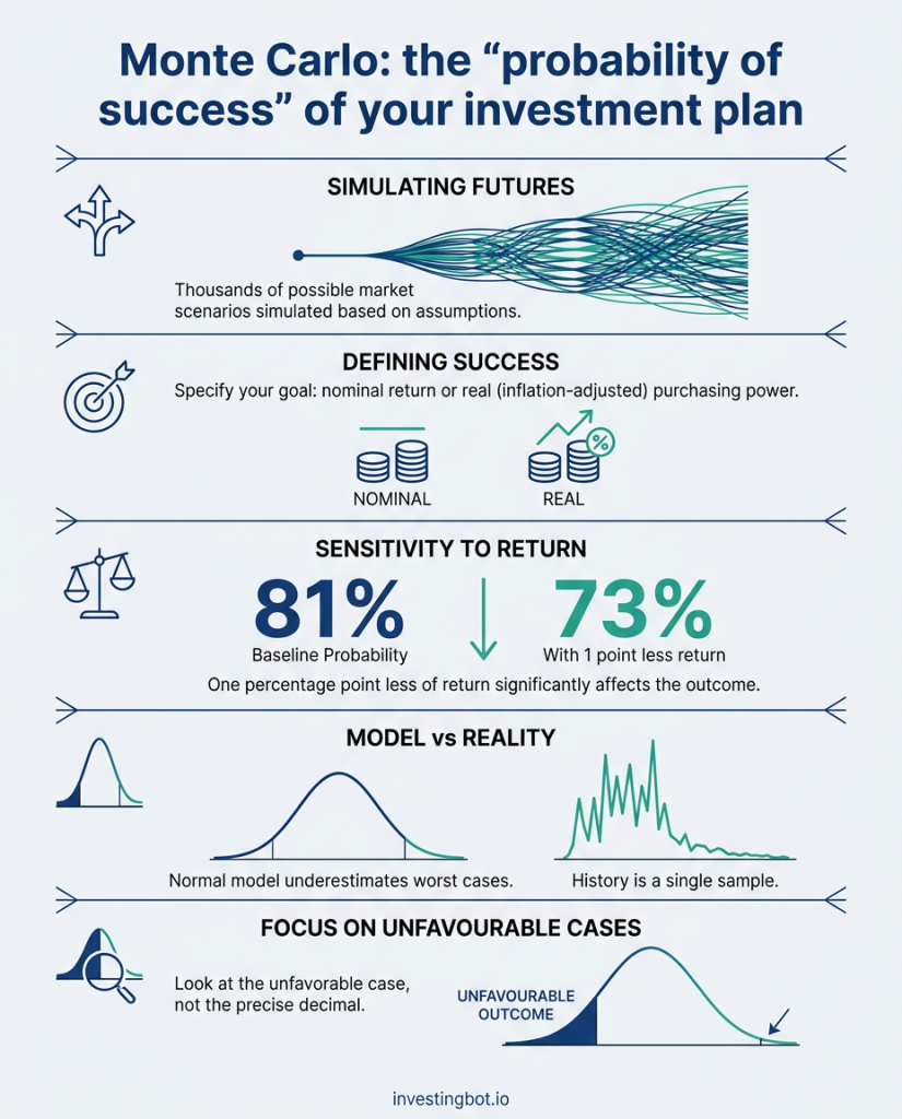
In short

• Monte Carlo tests a plan against thousands of possible futures generated from assumptions, and counts how often it reaches the goal.
• The “probability of success” depends on how success is defined, nominal or real, and over what horizon.
• In our data, one point less of return lowers the probability of reaching 1.5 times the money invested over 20 years from 81.3% to 72.7%.
• A model with independent months underestimates the worst cases: the block bootstrap shows them heavier.
• History is a single sample, and the US one is the most favourable among 39 markets.
• Read the range, above all the unfavourable case, not the decimal of the probability.

What is a Monte Carlo simulation in investing?

It is a method that tests an investment plan against thousands of randomly generated market paths, based on assumptions about return and volatility. For each path it calculates the final capital, and in the end it counts in what share of cases the goal was reached.

What does a 90% probability of success mean?

It means that, under the assumptions used, 90 simulated paths out of 100 reach the defined goal. It is neither a guarantee nor a forecast: it changes if the assumptions, the definition of success or the horizon change.

How much do the return assumptions matter?

A lot. In our data, lowering the real return by just one point a year reduces the probability of reaching 1.5 times the money invested over 20 years from 81.3% to 72.7%.

Is Monte Carlo more reliable than historical data?

Not necessarily. History is a single sample, with few truly independent long periods; Monte Carlo generates many, but only within the model’s assumptions. The block bootstrap, which reshuffles pieces of real history, is a compromise between the two.

Why are the worst cases often underestimated?

Because many models treat each month as independent of the previous one, while in reality negative periods often come in a row. In our data the worst 5% of 20-year outcomes starts from 1.11 times the money invested with the normal model and from 0.92 times with the block bootstrap.

How do I use Monte Carlo for my own plan?

Look at the unfavourable case and ask yourself whether you could live with it: if so, the plan is robust. Check that results are net of inflation and costs, and try more cautious return assumptions to see how much the result changes.